| 
|
||||||
Between Group Eigen Analysis of Microarray Data | |||||||
| BGA Web Tutorial |
|
|
|||||||
|
Home
Takes you to our home page Figures Figures from the paper Supplement Enhanced interactive Figures (Khan dataset) Method The mathematical basis of BGA ADE-4 - Download ADE-4 software |
Running BGA using ADE-4
This tutorial descibes how to run between group eigen analysis (BGA) using the multivariate software package ADE-4, which is freely available on Mac and Windows operating sytems. Preparing the dataStart up ADE-4. Use File -> Change data folder to specify the working directory (the folder in which your microarray data files are saved) Convert the raw data into binary format using by dragging and dropping onto the ADE-trans icon
The converted binary file can be viewed dragging and dropping it on the ADEBin icon 
Create a category file. This is a text file containing a one column list with the same number of rows as the data file. For example if you have 35 microarrays, this should contain 35 rows. This assigns each sample to a category (or grouping), thus if you have four data groups, it should contain a list of 1,2,3,4 where 1 assigns that sample to group 1, etc. Convert this file into binary format using ADETrans (as above). Then read this read, using CategVar->Read Categ File. 
Running the analysisThe data must be non-negative (usually integer) values for COA, if required a scalar can be added to the data using MatAlg -> Scalar Addition 
A standard COA will produce 8 output files (.fcta, .fcpl, .fcpc, .fcma, .fcvp, .fcpa, .fcli and .fcco) and a log file. Equally a PCA will produce 8 output files, these are labelled .cnXX where last two letters are the same as those from a COA. The .XXvp file contain the eigenvalues and relative inertia for each axis. The .XXco and .XXli contain column and row scores respectively. Note the naming convention: xxli (rows), .xxco (columns). Details about the output files are available in the ADE-4 help files, which can be accessed. from each menu. This outputs a .dis file which is the input file for between analysis. 
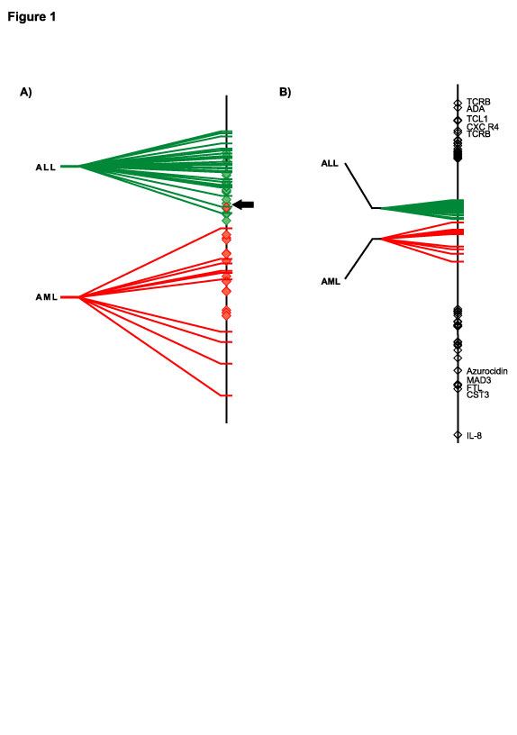
and then run between analysis Discrimin-> Between analysis:Run. A monte carlo test (permutation) test on the data can be run using Discrimin-> Between analysis:test. Between analysis producing 9 output files and a log file. These files are .bec1, .beco, .beli, .bels, .bepa, .bevp, .bepc, .bepl and .beta. Again the .XXvp file contains the eigenvalues and relative inertia for each axis. The .XXco contains the standard column scores (genes co-ordinates), the .beli contains the standard scores of the groups (centroids of the groups) and the .bels file contains the sampling unit scores resulting from the averaging on the column scores (individual sample co-ordinates). The .XXpl and .pc contain the weights of the groups and columns.Projecting Test dataPrepare the test data as above. Save test data as tab-delimited file with no column or row names. Convert to binary format (as above).Then use DDUtil ->Supplementary Rows to transform the data, similarly to the initial transformations. For example COA (chi-square) or PCA (column centre). Select the .XXvp file (.fcvp for COA or .cnvp for PCA) and your binary transposed test data. The number of rows must match. This will produce 2 files, the transformed data matrix (_tab) and another output file. Project the _tab file onto the BGA axis using DDUtil ->Row Projections. Select the .bevp file and the _tab file. This will produce one output file, which are the projections of the test data onto the bga axes. Graphing the resultsIf you have only two groups, this will produce one axis which discriminates between the two groups. A simple graph such as these can be produced using Graph 1D->Between Graph. To plot the samples and genes plot the .bels and .beco files. 
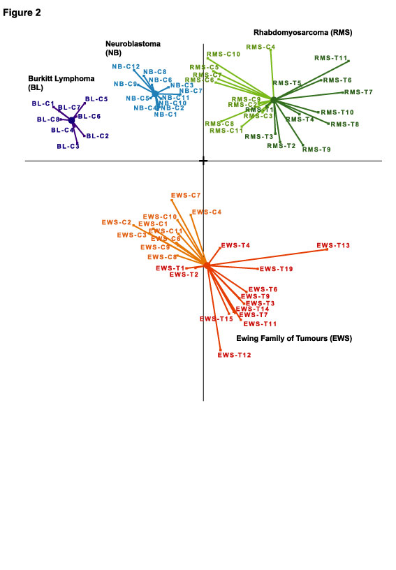
If you have more than one axis, use ScatterClass or Scatters, depending on whether you have category information (a .cat file) or not. ScatterClass->Stars will produce graph such as this. 
Again for more information on these modules, refer to the help provided in each menu |
||||||
| |||||||