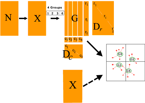
Mathematical basis of Between Group Eigenanalysis
BGA is carried out by ordinating groups (sets of grouped microarray samples) and then projecting the individual sample locations on the resulting axes. This is most easily done using PCA or COA. In this description, we will first describe COA and then show how we carry out the BGA on microarray data.
Correspondence analysis
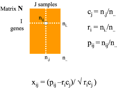
Consider a raw data table (N) of gene expression data for I genes (rows) and J microarray samples (columns) with elements nij. We denote the row sums and column sums of N as ni. and n.j respectively. The grand total of all the elements of N is denoted n..
The relative contribution or weight of gene i to the total variation in the data set is then denoted ri and is calculated as
ri = ni./n..
while the relative contribution of sample j is denoted as cj and is calculated as
cj = n.j/n..
Similarly, the contribution of each individual element of N to the total variation in the data set is denoted as pij and is calculated as
pij = nij/n..

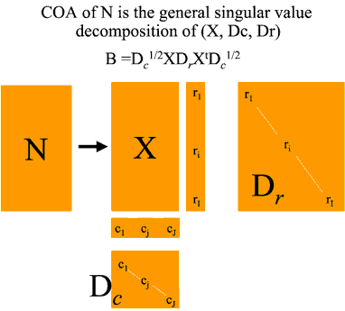
This produces two vectors R and C of length I and J and one IxJ matrix. We convert these into an IxJ table of chi squared values X using the forumla above. It is this table X that is analysed to produce the correspondence analysis. This table shows the associations between genes and samples. The total association between all genes and all samples is given by the total chi squared value for the data set (x..) which is the grand total of all the elements of X. COA then consists of decomposing this total chi squared into components for each gene and each sample along each of K eigenvectors where K is min(I-1,J-1). These eigenvectors are ranked according to their eigenvalues. The total of all the eigenvalues equals the total chi squared value for the data set. The actual method used in ADE-4 to derive the eigenvectors is general singular value decomposition (Dolédec and Chessel, 1987) where we calculate matrix B below as:

Here, Dc1/2 is a JxJ matrix with the square roots of the elements of C along the diagonal and zeros elsewhere. Similarly Dr is an IxI matrix derived from vector R with the elements of R along the diagonal and zeros elsewhere. Finally B is a JxJ matrix which is diagonalised to produce J eigenvalues (at least one of which will be zero) and eigenvectors.
The results of a COA are viewed by plotting the co-ordinates of all genes and samples along the top 2 or 3 eigenvectors. Groupings of samples or trends in the data set can be seen and interpreted using the proximity of genes and samples in plots as a guide. Samples and genes which are strongly associated, as measured by their chi squared values, will lie in a similar direction from the origin.
Between Group Eigenanalysis
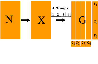
BGA is carried out where we can specify G groups of samples in advance. For example say we have four groups, then J columns (samples) will be grouped into four groups (G1-4).

The purpose of the analysis is then to ordinate these groups so as to separate them maximally in some space. This is achieved by grouping the J columns (samples) and calculating the vector C of column weights with G elements (4) where each element is the sum of column weights for one group i.e. Cg is the sum of the sample weights for group g.
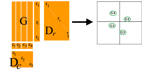
Matrix Dc then has GxG elements and the COA is carried out as before using using general singular value decomposition as above. The result of this is to produce G-1 eigenvectors with the co-ordinates of all genes and of the group centroids.

In this case we produce 3 axes which separate the four maximally in space. Finally, all individual samples are plotted on the G-1 eigenvectors as supplemental points.

See a tutorial for help on running BGA using ADE-4 or see the figures from the paper.
